Life in the Classic Maya Period: Majesty and Beauty
Apr 21, 2023
The Maya Classic period is widely considered the golden age of the ancient Maya and saw incredible achievements in art, architecture and science. Let’s explore what made this time period so brilliant and why the classic period continues to fascinate the scholars and public today.
Archaeologists use muography in Naples to reveal hidden chamber.
ARCHAEOLOGISTS USE MUOGRAPHY TO REVEAL HIDDEN CHAMBER IN NAPLES
A TEAM OF ARCHAEOLOGISTS HAVE USED MUOGRAPHY TO REVEAL A HIDDEN CHAMBER IN THE NECROPOLIS OF NEAPOLIS IN NAPLES, ITALY.
Neapolis was a Greek city founded during the 3rd century BC, whose remains are located around 10 metres beneath the current street level in the Sanità neighbourhood of present-day Naples.
The city emerged as an important trading centre in Magna Graecia and the Mediterranean, but would eventually be absorbed into the expanding Roman Republic around 327 BC.
The study was conducted by the University of Naples Federico II and the National Institute of Nuclear Physics (INFN), in collaboration with the University of Nagoya (Japan).
The team applied muography, a technique that uses cosmic ray muons to generate three-dimensional images of volumes using information contained in the Coulomb scattering of the muons.
Since muons are much more deeply penetrating than X-rays, muon tomography can be used to image through much thicker material than x-ray based tomography such as CT scanning.
Several detectors capable of detecting muons were placed underground in the highly populated “Sanità” district at a depth of 18 metres to measure the muon flux over several weeks.
Measurements of the differential flux in a wide angular range have enabled the researchers to produce a radiographic image of the upper layers that has revealed known and unknown structures beneath the ground surface.
One of the most interesting structures is an inaccessible hidden chamber from the Hellenistic period, which according to the researchers likely contains a burial.
“From the number of muons that arrive at the detector from different directions, it is possible to estimate the density of the material they have passed through,” said lead author Valeri Tioukov, a researcher at the INFN of Naples. “We found an excess in the data that can only be explained by the presence of a new burial chamber.”
We report in this paper the muography of an archaeological site located in the highly populated “Sanità” district in the center of Naples, ten meters below the current street level. Several detectors capable of detecting muons - high energy charged particles produced by cosmic rays in the upper layers of atmosphere - were installed underground at the depth of 18 m, to measure the muon flux over several weeks. By measuring the differential flux with our detectors in a wide angular range, we have produced a radiographic image of the upper layers. Despite the architectural complexity of the site, we have clearly observed the known structures as well as a few unknown ones. One of the observed new structures is compatible with the existence of a hidden, currently inaccessible, burial chamber.
Introduction
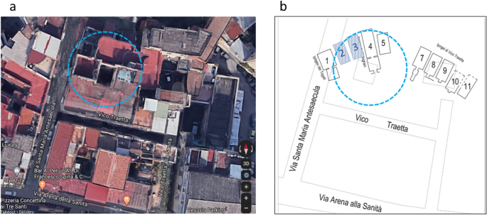
Remains of the ancient Neapolis with its buildings, streets, aqueducts and necropolis made by the Greeks starting from the second half of the first millennium BC are interred approximately ten meters below the current street level of the city of Naples. A little part of this archaeological treasure is accessible, thanks to the underground structures like water cisterns made since the sixteenth century or bomb shelters build during the Second World War which accidentally cross ancient cultural layers. Systematic archaeological excavations are not always possible in Naples, mainly because of safety concerns for buildings and streets in its highly populated districts. The Ipogei dei Togati and the Ipogei dei Melograni, denoted in Fig. 1 as chambers 1 and 4, respectively, are two known Greek burial chambers found below the Sanità district of Naples. The tombs are part of the ancient necropolis developed in this area in the VI–III century BC. Beautiful frescoes and alto-relievos were found in these ancient monuments created by wealthy Hellenistic families as shown in Fig. 2. In this area, covered later on by a thick alluvial layer hiding all memories of ancient preexistence, a fast-growing urbanization has been developing since the XVI century. The new constructions, while intersecting the ancient monuments, have often incorporated or partially destroyed them. Despite the profound transformations of this area over time, recent studies allowed to figure out the original morphology of the ancient necropolis landscape with burial chambers, developed along the road originating from the North Gate of Neapolis. The study of the integrated site topology with 3D surveys led to the hypothesis of a possible presence of additional burial hypogea as part of the Hellenistic necropolis, as shown in Fig. 1. In order to investigate this hypothesis, in this paper we have explored the site with the muon radiography technique. This modern technique consists of measuring the differential flux of muons, elementary particles naturally produced in the upper layers of the Earth atmosphere. The angular and momentum spectrum of muons, their flux, as well as their propagation length through different materials are well known. Therefore, this perpetual muon rain on the Earth surface can be used for the radiography, hence the so-called muography, of massive targets such as volcanoes 1,https://doi.org/10.1038/s41598-019-43131-8
(2017)." href="https://www.nature.com/articles/s41598-023-32626-0#ref-CR9" data-track="click" data-track-action="reference anchor" data-track-label="link" data-test="citation-ref" aria-label="Reference 9">9. Due to its non-invasive nature, this technique is particularly suitable for urban environments where the application of active inspection methods such as seismic waves or boreholing is not conceivable.
Figure 1
(a) Foreground top view of the studied site as seen with Google Maps https://www.google.com/maps accessed 22/06/2022
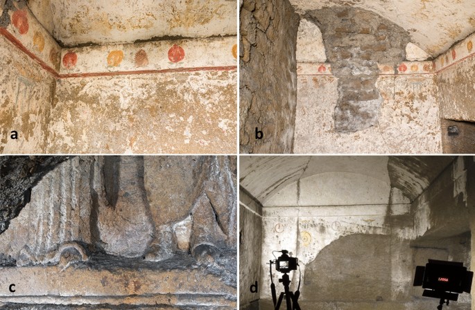
(a) Fragments of Greek burial chambers and (b) Ipogeo dei Melograni decorated with fruits frescoes along the walls (c) Togati - fragment of a high relief with a funeral farewell scene (d) chamber 8 in Fig. 11 with remains of frescoes on the North wall described by Neapolitan archaeologist Michele Ruggiero in 1888.
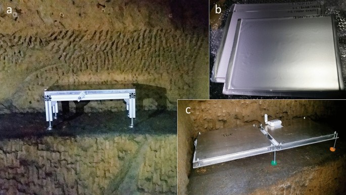
(a) Emulsion detector VP2 while taking data installed underground in the U15 “Chianca” room at 18 m depth. (b) Emulsion plates sealed inside protective envelopes.(c) Emulsion detector VP1 taking data in parallel in a different position inside the same cellar. The total sensitive area of each detector is 1500http://www.w3.org/1998/Math/MathML"><mtext> </mtext><mi>c</mi><msup><mi>m</mi><mn>2</mn></msup></math>">cm2 ��2.
We have used a detector based on the nuclear emulsion technology 10, featuring the highest spatial resolution in measuring ionizing particle tracks. Nuclear emulsion is composed of tiny silver bromide crystals immersed in a gelatin binder. The crystals act as sensors that are activated by the ionization loss of a passing-through charged particle. The activated state of the crystals is preserved until the emulsion film is chemically developed. Thus, a particle track is recorded, first as a sequence of activated crystals, which later, after the development, becomes a sequence of silver grains. The formed tracks are visible at fully automated optical microscopes where their position and direction are measured.
Emulsion detectors are simple, extremely compact and, unlike electronic detectors, they don’t require any power supply 10 or gas feeding system. This makes them particularly suitable in a harsh environment such as in underground installations or on volcanoes. We used two detector modules shown in Fig. 3 and assembled with the same structure, consisting of a pile of four films, http://www.w3.org/1998/Math/MathML"><mn>25</mn><mo>×</mo><mn>30</mn><mtext> </mtext><mi>c</mi><msup><mi>m</mi><mn>2</mn></msup></math>">25×30cm225×30 ��2 wide and about 300 http://www.w3.org/1998/Math/MathML"><mi>μ</mi></math> ;">μ�m thick. Each emulsion film was sealed inside an envelope for light and humidity tightness. The film piles were placed between two flat aluminum plates, acting both as protection layers and as the mechanical frame of the detector. A thin soft rubber layer was added between the top plate and the emulsion film to distribute uniformly the pressure and protect sensitive layers against any mechanical stress.
Figure 5
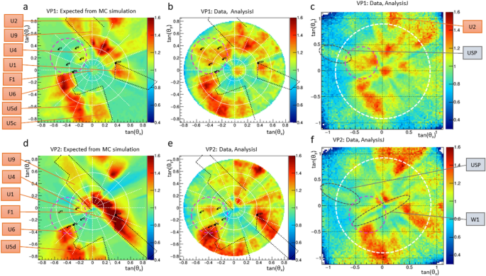
Muography images reporting the muon flux simulated using the 3D model (a,d) and measured (b,c,e),f) all normalized to the one obtained by MC at the detector depth in the assumption of a bulk rock. Color scale represents the relative flux excess with respect to the one without cavities. (a–c) show the expected and measured AnalysisI and AnalysisJ, respectively, for the VP1 while (d–f) show the same quantities for the VP2. The white dashed circle in the (c, f) plots shows the angular acceptance of the AnalysisI.
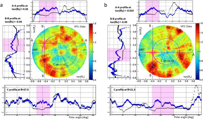
(a) The plot in the center is the bi-dimensional muography plot, same as in Fig. 5b. (b) The plot in the center is the same as in Fig. 5e. Both plots are accompanied with 3 profiles corresponding to the section lines A-A. B-B and the circumference C. Solid pink segments indicate the anomaly span. On the profile plots these regions are highlighted, the blue line stay for data, black for simulation (shown on Figs 5a and 5d), the vertical error bars represent the statistical uncertainties defined by the bins population with muons. The angles are given in degrees (0–360), the polar one follows east-counterclockwise convention.
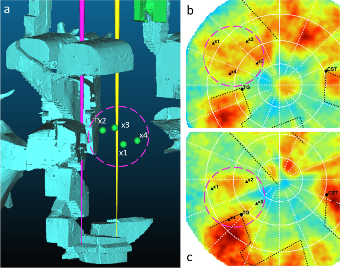
(a) 3D view of the site with the four inferred reference pointshttp://www.w3.org/1998/Math/MathML"><msub><mi>x</mi><mn>1</mn></msub></math> ;">x1�1tohttp://www.w3.org/1998/Math/MathML"><msub><mi>x</mi><mn>4</mn></msub></math> ;">x4�4reported as green spheres. (b,c) are the zoomed view of the region of interest as seen from the two detectors. Black triangles present the projections on the muography image of the 3D pointshttp://www.w3.org/1998/Math/MathML"><msub><mi>x</mi><mn>1</mn></msub></math> ;">x1�1tohttp://www.w3.org/1998/Math/MathML"><msub><mi>x</mi><mn>4</mn></msub></math> ;">x4�4.
The modules were kept horizontally for 28 days in the period March 10 to April 7, 2018 inside the so-called “Chianca” underground room, a cellar used in XIX century for ham aging, denoted as U15 in this work, at a depth of about 18 m below the street level. At the end of the exposure the piles were disassembled and the films were kept in a different order during their transportation. Emulsion films register all the charged particles crossing the sensitive layers until they are developed. In a single emulsion plate tracks registered during the exposure period cannot be distinguished from those integrated elsewhere. To solve this ambiguity, we typically use a stack of two or more emulsion films placed in a given order and the pattern matching procedure to identify those tracks integrated during the exposure. This procedure shows a purity higher than 95%.
All emulsions were developed in Naples next day after the detector extraction.
Normally two consecutive plates are sufficient for unambiguous reconstruction. In this experiment stacks of four films were divided in two doublets. Each doublet was independently analysed in one of the two scanning laboratories equipped with high performance scanning systems: Naples (Italy) and Nagoya (Japan). Both the scanning and analysis chains applied in two laboratories were independent. The final results are fully compatible, confirming the high quality of both processing. To distinguish between these two analysis chains, hereafter we refer to AnalysisI and AnalysisJ for Naples and Nagoya, respectively.
Digital model of the site
As it is the case for medical X-ray radiography where the recognition of anomalies relies on the precise knowledge of the body structure, also for the muon radiography the recognition of hidden hollow structures requires a 3D model of the known structures. This is particularly important in the investigation of such a complex and multi-layer environment of the underground structure of Naples. There are stairs and cisterns spanned from the depth of 20 m up to the surface level; the historical layer, target of this investigation, is at the depth of http://www.w3.org/1998/Math/MathML"><mn>8</mn><mo>÷</mo><mn>12</mn></math> ;">8÷128÷12 m; concrete basements of the buildings are rising up from the depth of about 6 m; cellars, underground sewer and connections, street level structures and the buildings themselves have to be described in the model.
Table 1 List of all accessible underground structures.
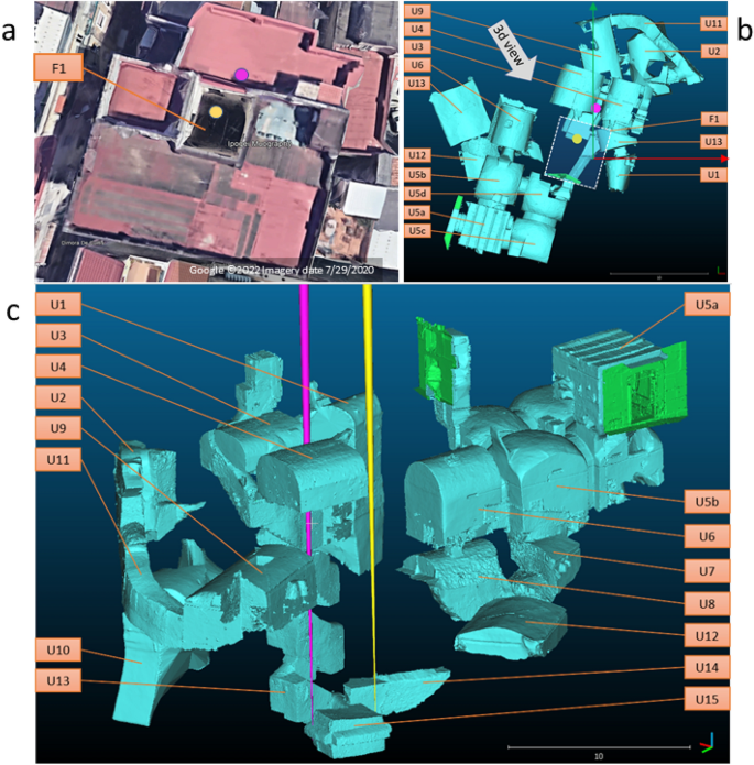
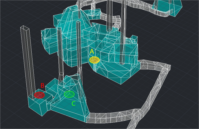
Muography produces overlaid images of all the layers above the detector position, making the detection of unknown structures rather challenging. A dedicated laser scanning campaign was carried out by the ACAS3d company in this work, as part of the Italian cultural heritage program for digitizing historical and archaeological monuments. The survey was extended to all ancillary underground spaces such that a precise spatial model containing all the accessible underground structures was produced, as shown in Fig. 4. This figure shows both foreground (a), and underground (b) and (c) parts of the site. Moreover, narrow cones with their vertices in the center of the detector and their axis along the vertical direction are drawn to indicate the two detectors and their prospective views: hereafter we identify the detector positions (View Points) as VP1 and VP2, corresponding to yellow and purple cones respectively. In order to easy the navigation across the site and in the following plots, we have assigned in Table 1 a unique identifier to all the known underground locations. This 3D model of the site was introduced in a Geant4 based simulation to describe the particle propagation through matter and produce the expected muon flux at the detector. This procedure is described in detail in the “Methods” Section.
Data compared with the expectation from known structures
The plots in Fig. 5 show the expected (a, d) and measured (b,c,e,f) muon flux, all normalised to the flux obtained by MC at the detector depth in the assumption of a uniform bulky rock with no cavities, as a function of the projected slopes of the muon tracks, i.e. http://www.w3.org/1998/Math/MathML"><mi>tan</mi><mo></mo><mrow class="MJX-TeXAtom-ORD"><msub><mi>θ</mi><mi>x</mi></msub></mrow><mo>=</mo><mrow class="MJX-TeXAtom-ORD"><mi mathvariant="normal">Δ</mi><mi>x</mi></mrow><mrow class="MJX-TeXAtom-ORD"><mo>/</mo></mrow><mrow class="MJX-TeXAtom-ORD"><mi mathvariant="normal">Δ</mi><mi>z</mi></mrow></math>">tanθx=Δx/Δztan��=Δ�/Δ� and http://www.w3.org/1998/Math/MathML"><mi>tan</mi><mo></mo><mrow class="MJX-TeXAtom-ORD"><msub><mi>θ</mi><mi>y</mi></msub></mrow><mo>=</mo><mrow class="MJX-TeXAtom-ORD"><mi mathvariant="normal">Δ</mi><mi>y</mi></mrow><mrow class="MJX-TeXAtom-ORD"><mo>/</mo></mrow><mrow class="MJX-TeXAtom-ORD"><mi mathvariant="normal">Δ</mi><mi>z</mi></mrow></math>">tanθy=Δy/Δztan��=Δ�/Δ� where z is vertical (Zenith) axis. The expected flux at the location of our detectors, at the depth of 18 m, is obtained by including in the simulation the detailed 3D model reported in the previous Section. Top plots in Fig. 5 are for VP1, bottom plots for VP2.
These plots provide a view of the site similar to that one could take with a camera installed at the same location of our detectors, if rocks were partially opaque to the visible light, the opacity being proportional to the rock density. The color scale shows the amplitude of the flux ratio: the green color (ratio approximately equal to 1) indicates a muon flux compatible with the hypothesis of no-cavity in the given angular bin while a yellow-red color shows an excess due to cavities intercepted by the particles coming from those directions. The images of the most relevant underground structures are clearly visible here and are marked with corresponding identifiers. Black dashed contours are projections of the 3D lines indicating the shapes of some structures: U5, U6, U9 (Melograni) and U1 (cistern). Comparing left and right plots, one can clearly see the very close similarities of most of the structure shapes such as U5, U6, and U1. Not all regions show a perfect correspondence between data and expectations, due to some missing details such as the density variation in the underground layers and the wastewater network under the street. The most important missing details are load-bearing walls and the concrete foundations of buildings. These details contribute to the suppression of the muon flux especially in the low angle region, within 10 degrees from the vertical direction. In particular, the VP2 happens to be below the load-bearing wall of the building, and this is clearly visible in the plots (e, f) where the hardly suppressed region in the center is highlighted by a dashed grey ellipse “W1”.
Table 2 Positions of the detectors and coordinates of reference points in the reference system used in the paper (in meters).
Apart from these differences attributed to some details missing in the 3D model, the most interesting anomaly detected in this analysis is the one inside the pink dashed circle drawn on all 6 plots between U6 and U4. There is no known structure expected to produce an increase in the muon rate in the region on the left of U4 as it is visible in the plots (a and d). Nevertheless, a clear excess in that region is found in the data, and reported in the plots (b, c, e and f). The reference points http://www.w3.org/1998/Math/MathML"><msub><mi>x</mi><mn>1</mn></msub></math> ;">x1�1, http://www.w3.org/1998/Math/MathML"><msub><mi>x</mi><mn>2</mn></msub></math> ;">x2�2, http://www.w3.org/1998/Math/MathML"><msub><mi>x</mi><mn>3</mn></msub></math> ;">x3�3, http://www.w3.org/1998/Math/MathML"><msub><mi>x</mi><mn>4</mn></msub></math> ;">x4�4 on (a, b, d, e) indicate the boundaries of this region, as projections of 3D points on both VP1 and VP2 muographies. These 3D points are denoted as small green spheres in the 3D view of the site reported in the a) picture of Fig. 7. Plots (b) and (c) in the same Figure show a zoomed view of the anomaly region for both muographies. The observed excess is compatible with a cavity http://www.w3.org/1998/Math/MathML"><mn>2</mn><mo>÷</mo><mn>3</mn></math> ;">2÷32÷3 m height, located in the volume delimited by the http://www.w3.org/1998/Math/MathML"><msub><mi>x</mi><mn>1</mn></msub><mo>−</mo><msub><mi>x</mi><mn>4</mn></msub></math> ;">x1−x4�1−�4 points. The coordinates of reference points and the detector positions in the 3D-model reference system aligned with data are summarized in Table 2. The mean depth of the anomaly is of 8.5 m below the surface and the distance between points is http://www.w3.org/1998/Math/MathML"><mn>2</mn><mo>÷</mo><mn>3.5</mn></math> ;">2÷3.52÷3.5 m, which characterize the cavity dimension. The projection of the anomaly to the muography shown in plot b) is partially superimposed to U4 while in plot c) there is a partial overlap with U6 located on the upper levels. In the plot c) of Fig. 7, it can be seen that there is a region where the muon flux is suppressed: this region marked as W1 on Fig. 5f spans radially from the center toward the left bottom quadrant dividing the anomaly into two parts one identified by http://www.w3.org/1998/Math/MathML"><msub><mi>x</mi><mn>1</mn></msub></math> ;">x1�1 and http://www.w3.org/1998/Math/MathML"><msub><mi>x</mi><mn>2</mn></msub></math> ;">x2�2, and the other one with http://www.w3.org/1998/Math/MathML"><msub><mi>x</mi><mn>3</mn></msub></math> ;">x3�3 and http://www.w3.org/1998/Math/MathML"><msub><mi>x</mi><mn>4</mn></msub></math> ;">x4�4, due to the shadow effect of the load-bearing wall of the building located just above VP2.
Discussion
The comparison between the measured and expected muon flux shown in Figs. 5 and 7 provides the evidence for a new empty structure and allows to estimate its size and position.
In Fig. 6 we report the profile plots for data (blue) and simulation (black) in order to better investigate the anomaly shape and its statistical significance. The highlighted regions correspond to the anomaly span indicated also by solid pink lines on the 2d plots. The error bars shows the statistical uncertainty derived from http://www.w3.org/1998/Math/MathML"><mn>1</mn><mrow class="MJX-TeXAtom-ORD"><mo>/</mo></mrow><msqrt><mi>n</mi></msqrt></math>">1/n−−√1/� where n is the number of muons per bin in the plots of Fig. 5. Since the statistics in the simulation was one order of magnitude higher than in the data, black line errors are negligible. In the anomaly region highlighted on the profile plots, the excess is clear on all profiles and cannot be explained by the statistical uncertainty. Thanks to the high statistical significance of each bin we can observe clearly the shape of the structures on the 2d distributions. In the other regions, a very good agreement is in general visible which supports a good description of the existing structures. The observed deviations of data plots from simulated ones reflect the difference in terms of shape and/or material density between the real site structure and the 3D-model used for the simulation. The excess in the simulation is clearly attributed to the shadow effect of the building walls missing in the model. There is another excess region in the data possibly due another unknown cavity which is less evident and revealed only in one projection, not sufficient for a 3D position estimation.
The anomaly location is consistent with the existence of a burial chamber, denoted as number 3 in Fig. 1, likely to be partially filled with alluvial material. The size of this empty region is expected to be http://www.w3.org/1998/Math/MathML"><mn>2</mn><mo>÷</mo><mn>3.5</mn></math> ;">2÷3.52÷3.5 m. The anomaly is clearly visible and its location is well-defined. The projection to the muography space tends to distort rectangular shapes, expected for a burial chamber, into quadrilateral shapes. In fact, we see a quadrilateral shape, thus indicating a structure of anthropogenic origin, consistent with a new burial chamber.
From the comparison of data with the expectations in all the other angular regions in Fig. 5, one can observe in general a very good agreement, with all the known structures detected. Nevertheless, there are regions where differences between data and simulation are visible. These differences can be attributed to the accuracy of the simulation model, due to the following reasons:
No structural model of the nearby buildings, including their load-bearing walls, basements or other massive elements is available.
The empty space is described with a null density while the rock with the constant value of 2.0 g/cmhttp://www.w3.org/1998/Math/MathML"><msup><mi></mi><mn>3</mn></msup></math> ;">33. This is a rough approximation as some underground regions are dominated by volcanic tuff, others by diluvial material while buildings basements are made of concrete. The actual density of these materials ranges between 1.4 and 2.4 g/cmhttp://www.w3.org/1998/Math/MathML"><msup><mi></mi><mn>3</mn></msup></math> ;">33.
Not all empty underground spaces are described in our model. Underground connections, sewerage tombs and pipes are missing. It is also possible that some cellars of nearby buildings are missing from the model even though they lie within the acceptance region of the detectors.
These effects produce the small discrepancies between the expected and measured muon rates observed in some angular regions. Nevertheless, the size of these discrepancies cannot explain the observed anomaly. Firstly, the building walls create a sizeable effect when placed just above the detector since the muons travel a path as long as several meters inside the wall material. In this case the muon flux is strongly suppressed and a “shadow” is observed along this direction. This is the reason why a linear structure crossing the anomaly is visible in the plots (e, f) of Fig. 5. This effect is expected to decrease with the angle, and indeed it becomes negligible above 10 degrees. Secondly, soil density uncertainties result in a slight deviation of the rate in some angular regions but cannot produce a room-shaped anomaly. The cavity at the depth of 10 meters could not be confused with a cellar missing in the model, as they are typically located at the depth of 2–4 meters. Finally, the effect of missing pipelines or underground connections could result in a thin linear structure, incompatible with the observed anomaly. In fact we observe this kind of structure developing linearly toward the outer angular regions, marked as USP (Under Surface Pipeline) on Fig. 5c,f.
The reconstruction accuracy of the observed cavity could in principle improve by taking images from different angles, thus producing a tomography of the site. Nevertheless, the difficulty lies in the accessible sites for detector installations which are extremely limited in situ. The imaging of the site reported in this paper can thus be considered an optimal one.
Methods
Emulsion data reconstruction
The emulsion films used for this experiment were produced at Nagoya University. Each films is http://www.w3.org/1998/Math/MathML"><mn>25</mn><mo>×</mo><mn>30</mn></math> ;">25×3025×30 cmhttp://www.w3.org/1998/Math/MathML"><msup><mi></mi><mn>2</mn></msup></math> ;">22 and consists of two sensitive layers, 70 http://www.w3.org/1998/Math/MathML"><mi>μ</mi></math> ;">μ�m thick each, deposited on both sides of a 175 http://www.w3.org/1998/Math/MathML"><mi>μ</mi><mi>m</mi></math> ;">μm�� thick polystyrene base https://doi.org/10.1002/9781119722748.ch21
(Wiley, 2022)." href="https://www.nature.com/articles/s41598-023-32626-0#ref-CR11" data-track="click" data-track-action="reference anchor" data-track-label="link" data-test="citation-ref" aria-label="Reference 11">11. AgBr crystals have a diameter of about 200 nm and the expected grain density for minimum ionizing particles tracks is on average about 40 grains per 100 http://www.w3.org/1998/Math/MathML"><mi>μ</mi></math> ;">μ�m path. After the emulsion development the grains size is of 0.6 http://www.w3.org/1998/Math/MathML"><mi>μ</mi></math> ;">μ�m. The readout of emulsion detectors requires high performance Scanning Systems https://doi.org/10.1016/j.nima.2005.06.072
(2005)." href="https://www.nature.com/articles/s41598-023-32626-0#ref-CR12" data-track="click" data-track-action="reference anchor" data-track-label="link" data-test="citation-ref" aria-label="Reference 12">12,13 (SS), fully automated microscopes equipped with digital cameras and image processing chains. The whole thickness of the sensitive layers is spanned by adjusting the focal plane of the objective lens and a sequence of several tens of tomographic images is taken for each field of view at equally spaced depth levels. Emulsion images are then digitized, converted into a grey scale of 256 levels, sent to a vision processor board and analyzed to recognize sequences of aligned grains, i.e. clusters of dark pixels of given shape and size. Some of these spots are track grains; others, in fact the majority, are grains not associated to muon tracks, but rather to Compton electrons or produced by thermal excitation. The three-dimensional structure of a track in an emulsion layer (microtrack) is reconstructed by combining clusters belonging to images at different levels and searching for geometrical alignments. Each microtrack pair is finally connected across the plastic base to form the so-called base track. The typical resolutions for this type of emulsions in the detection of high energy (>1 GeV) charged tracks is of about 1 http://www.w3.org/1998/Math/MathML"><mi>μ</mi></math> ;">μ�m in position, 1.5 mrad in the http://www.w3.org/1998/Math/MathML"><mi>ϕ</mi></math> ;">ϕ� angle and from 1.5 to 6 mrad depending on http://www.w3.org/1998/Math/MathML"><mi>θ</mi></math> ;">θ� for the radial angle component 14. So even a single 300 http://www.w3.org/1998/Math/MathML"><mi>μ</mi></math> ;">μ�m thick emulsion plate provides remarkably high angular resolution sufficient for most of muography applications. A detector module typically consists of at least two consecutive plates for the purpose of separating particle tracks integrated during exposure runs from other tracks. Reconstruction of a long track crossing several plates normally leads to an improvement in angular resolution. The next step is a pattern recognition procedure where the alignment of consecutive films with micrometric accuracy is achieved https://doi.org/10.1016/j.nima.2005.11.214
(2006)." href="https://www.nature.com/articles/s41598-023-32626-0#ref-CR15" data-track="click" data-track-action="reference anchor" data-track-label="link" data-test="citation-ref" aria-label="Reference 15">15. The reconstruction efficiency depends on the emulsion thickness, grain density and the exposure conditions and in this experiment was higher than 94%. A small dependency of the efficiency on the http://www.w3.org/1998/Math/MathML"><mi>θ</mi></math> ;">θ� angle is corrected in the post-processing phase. Two independent reconstruction and analysis chains were applied to different emulsion doublets. The SS used for AnalysisIhttps://doi.org/10.1088/1748-0221/11/06/P06002
(2019)." href="https://www.nature.com/articles/s41598-023-32626-0#ref-CR19" data-track="click" data-track-action="reference anchor" data-track-label="link" data-test="citation-ref" aria-label="Reference 19">19 are different from those employed in AnalysisJhttps://doi.org/10.1093/ptep/ptx131
(2017)." href="https://www.nature.com/articles/s41598-023-32626-0#ref-CR20" data-track="click" data-track-action="reference anchor" data-track-label="link" data-test="citation-ref" aria-label="Reference 20">20,21 in all respects, from hardware to software tools and track reconstruction algorithms. However, the final detection efficiency is similar and the angular distribution of muon tracks are fully compatible.
Angular acceptance for the emulsion detectors
Emulsion films register all charged particles passing through it, at any direction. As a result of the geometrical acceptance, the particle flux of muons crossing any flat surface decrease with the http://www.w3.org/1998/Math/MathML"><mi>θ</mi></math> ;">θ� angle as http://www.w3.org/1998/Math/MathML"><msub><mi>F</mi><mn>0</mn></msub><mi>cos</mi><mo></mo><mi>θ</mi></math> ;">F0cosθ�0cos�, where http://www.w3.org/1998/Math/MathML"><msub><mi>F</mi><mn>0</mn></msub></math> ;">F0�0 is the flux orthogonal to the surface (http://www.w3.org/1998/Math/MathML"><mi>θ</mi><mo>=</mo><mn>0</mn></math> ;">θ=0�=0). Since http://www.w3.org/1998/Math/MathML"><mi>θ</mi></math> ;">θ� regions close to http://www.w3.org/1998/Math/MathML"><mi>π</mi><mrow class="MJX-TeXAtom-ORD"><mo>/</mo></mrow><mn>2</mn></math>">π/2�/2 (parallel to plate) show low significance due to the geometrical acceptance, upper limits on the http://www.w3.org/1998/Math/MathML"><mi>θ</mi></math> ;">θ� range are normally applied in tracking algorithms, to reduce the processing time which is typically proportional to the solid angle, http://www.w3.org/1998/Math/MathML"><mn>2</mn><mi>π</mi><mo stretchy="false">(</mo><mn>1</mn><mo>−</mo><mi>cos</mi><mo></mo><mrow class="MJX-TeXAtom-ORD"><mi>θ</mi></mrow><mo stretchy="false">)</mo></math>">2π(1−cosθ)2�(1−cos�). This limit is set at http://www.w3.org/1998/Math/MathML"><mi>tan</mi><mo></mo><mi>θ</mi><mo>≤</mo><mn>0.8</mn></math> ;">tanθ≤0.8tan�≤0.8 (round cut) for AnalysisI and http://www.w3.org/1998/Math/MathML"><mo stretchy="false">(</mo><mi>tan</mi><mo></mo><msub><mi>θ</mi><mi>x</mi></msub><mo>≤</mo><mn>1.2</mn><mo stretchy="false">)</mo><mi mathvariant="normal">&</mi><mo stretchy="false">(</mo><mi>tan</mi><mo></mo><msub><mi>θ</mi><mi>x</mi></msub><mo>≤</mo><mn>1.2</mn><mo stretchy="false">)</mo></math>">(tanθx≤1.2)&(tanθx≤1.2)(tan��≤1.2)&(tan��≤1.2) (square cut) for AnalysisJ. The two analyses differ also in the bin size of the angular histograms. In AnalysisI, a bi-dimensional squared bin with 0.01 bin size in the tangent space is used followed by a smoothing of the resulting histograms. In the AnalysisJ, the bin size is 0.025 without smoothing. The smoothing procedure is equivalent to a low-pass filtering with a http://www.w3.org/1998/Math/MathML"><mn>3</mn><mo>×</mo><mn>3</mn></math> ;">3×33×3 core as used in image or signal processing to emphasise weak and wide signals: this first allowed to detect the cavity. On the other hand, the approach without smoothing does not introduce any distortion: sharp details such as wall shadows or room angles retain their original shape. Bin size selection depends also on the statistics. For the bin size of 0.01, significantly larger than the angular resolution quoted above, the statistics integrated in each bin is still sufficient: bins contained between 100 and 500 entries, in the peripheral (http://www.w3.org/1998/Math/MathML"><mi>tan</mi><mo></mo><mi>θ</mi><mo>=</mo><mn>0.8</mn></math> ;">tanθ=0.8tan�=0.8) and in the central (http://www.w3.org/1998/Math/MathML"><mi>tan</mi><mo></mo><mi>θ</mi><mo>=</mo><mn>0</mn><mo stretchy="false">)</mo></math>">tanθ=0)tan�=0)) regions, respectively. The total accumulated statistics for each detector is 5 and 7 millions of tracks in the AnalysisI and in the AnalysisJ correspondingly in 28 days of exposure.
Coordinate system for data presentation
There are several ways, i.e. coordinate systems, used for the presentation of muography data. In this paper, we have adopted the projected angular slopes of reconstructed muon tracks, http://www.w3.org/1998/Math/MathML"><mi>tan</mi><mo></mo><msub><mi>θ</mi><mi>x</mi></msub></math> ;">tanθxtan�� versus http://www.w3.org/1998/Math/MathML"><mi>tan</mi><mo></mo><msub><mi>θ</mi><mi>y</mi></msub></math> ;">tanθytan��, since they provide an intuitive picture, similar to the perspective projection used in conventional photographs. In doing that, the topology of the structures is approximately conserved and the comparison with an orthogonal site map becomes straightforward. Nevertheless, the binning inequality leads to a statistical suppression in the large http://www.w3.org/1998/Math/MathML"><mi>θ</mi></math> ;">θ� regions due to the solid angle effect proportional to http://www.w3.org/1998/Math/MathML"><mn>1</mn><mrow class="MJX-TeXAtom-ORD"><mo>/</mo></mrow><mi>c</mi><mi>o</mi><msup><mi>s</mi><mn>2</mn></msup><mi>θ</mi></math>">1/cos2θ1/���2�. This may makes the interpretation of results more difficult in those regions without normalization. This is why we report the flux ratio, observed over expected.
Cavity position determination and reference points
The method used relies on the assumption that the trapezoidal contour of the observed structure in the angular space as reported in Fig. 5 keeps the same topological shape when seen from the two detector sites, except for some shift, rotation and deformation. Therefore, one can associate in the angular space the coordinates of the four corners observed from the two detectors: e.g. http://www.w3.org/1998/Math/MathML"><msub><mi>x</mi><mn>1</mn></msub></math> ;">x1�1 denotes the same corner in both detector views. For each corner, we have drawn in the 3D space two lines, one for each detector, originated from the detector position with the slopes defined by the corners themselves. We have then computed the points belonging to the two lines associated with the distance of closest approach and then we have computed the average point between the two. The same procedure is carried out for all 4 corners. The resulting points are the ones denoted as http://www.w3.org/1998/Math/MathML"><msub><mi>x</mi><mn>1</mn></msub></math> ;">x1�1...http://www.w3.org/1998/Math/MathML"><msub><mi>x</mi><mn>4</mn></msub></math> ;">x4�4 in Fig. 5 and Fig. 7. The uncertainty estimated by the above procedure is of 0.5 m in XY and 1.2 m in Z coordinate.
Muons flux generation and plots normalization
Muons are charged particles mostly produced by the decay of pions copiously produced in the interaction of high-energy cosmic rays (mainly protons) with the nucleons contained in the upper layers of the Earth atmosphere. The flux at the sea level is approximately uniform and constant, with small time and coordinate dependent variations, of the order of 5%. These variations affects mainly the low-momentum part of the spectrum, below 1 GeV, which does not impact our measurements because they do not reach our detector anyway.
There are several models describing the atmospheric muon flux and their spectrum. In the AnalysisJ the Miyake 22 parametrization was used, for the AnalysisI the Bogdanova’s https://doi.org/10.1134/S1063778806080047
(2003)." href="https://www.nature.com/articles/s41598-023-32626-0#ref-CR24" data-track="click" data-track-action="reference anchor" data-track-label="link" data-test="citation-ref" aria-label="Reference 24">24, from the detector position towards the sky. This approach of inverse propagation simplified and sped up the simulation. Two cases were simulated: a flat monolithic rock layer of 18 m depth above of the detectors without any building and any cavity; the complete 3D underground model with all known cavities and buildings. The inner structure of buildings was not available, so they were approximated by solid blocks with an average density equal to 6% of the concrete one. The muon flux expected with all building implemented as well as the observed data were normalized to the flux one would get with the bulky rock model. This ratio is shown as a function of the projected angular slopes in Fig. 5, where the relative excess in the flux caused by underground cavities and foreground buildings is clearly seen. This plot could be interpreted as a kind of picture of the internal structure where empty volumes appears in a yellow-red color while dense volumes in a green–blue one. The adopted normalization corrects binning-related http://www.w3.org/1998/Math/MathML"><mi>θ</mi></math> ;">θ� dependencies and improves the sensitivity to deviations of the muon flux from its mean value.
Muography (or muon radiography) is a technique that exploits the penetration capability of muons, elementary particles similar to electrons but with a mass about 200 times larger. High energy muons are naturally produced in the interactions of cosmic rays with the Earth atmosphere. The measurement of their absorption in matter allows the imaging of the inner structure of large bodies. The technological developments in the detection of elementary particles have opened the way to its application in various fields, such as archaeology, studies of geological structures, civil engineering and security issues. We have developed a new approach to the three-dimensional muography of underground structures, capable of directly localising hidden cavities and of reconstructing their shape in space. Our measurements at Mt. Echia, the site of the earliest settlement of the city of Naples in the 8th century BC, have led us to the discovery of a hidden underground cavity, whose existence was not evident with the usual two-dimensional muography graphs. We demonstrate here that our original approach definitely enhances muography discovery potential, especially in case of complex underground systems.
Introduction
In all fields, imaging techniques capable of seeing inside physical bodies have brought an extraordinary progress to the power of investigation procedures. Muography is an imaging technique that profits from the penetrating power of elementary particles called muons, similar to electrons but with a mass about two hundred times larger. Muons are naturally produced in the interactions of cosmic rays with the Earth atmosphere. A conspicuous flux of muons is constantly hitting the Earth surface from all directions, from the Zenith to almost horizontal, providing an abundant “light” source for muography.
In absorption muography, a muon tracker is located downstream of the body under investigation. By tracking back the muon trajectories, one obtains an angular map of their flux as seen from the location of the muon tracker itself. A comparison with the muon flux impinging on the Earth surface provides a map of the muon transmission (or equivalently absorption) in the traversal of the body being investigated. As the penetration of muons in matter depends on its density, such a map can provide a muographic image of its internal structures. These could be cavities or high-density zones. Muography (or muon radiography) is thus in principle similar to X-ray radiography, but capable of probing the interior of large bodies, thanks to the penetrating power of muons which is much higher than that of X-rays.
The first muography was performed by the Nobelist Louis Alvarez in 1970, who disproved the possible existence of a hidden burial chamber in Chefren’s Pyramid1. Almost forty years later, muography was applied to the investigation of the inner structures of volcanic edifices2,3,4,5,6,7,8,9,10,11,12,13, facing the challenge posed by the observation of the low muon fluxes surviving the traversal of a large rock thickness typical of this application. However, the problem of low fluxes does not affect a very wide range of applications (from archaeology to risk assessment and prevention in civil engineering or geology), where the thickness of matter being traversed is at most several tens of meters14,15,16,17,18,19,20,21,22. The results obtained by the ScanPyramids project at the Khufu’s Pyramid23 and by our group in exploring underground cavities at Mt. Echia in ancient Napleshttps://doi.org/10.1038/s41598-017-01277-3
(2017)." href="https://www.nature.com/articles/s41598-019-39682-5#ref-CR24" data-track="click" data-track-action="reference anchor" data-track-label="link" data-test="citation-ref" aria-label="Reference 24">24 belong to this domain.
Mt. Echia (also called Pizzofalcone) is the site of the earliest settlement of the city of Naples in 8th century BC. It is a headland with a maximum altitude of about 60 m a.s.l. and mainly consists of yellow tuff, a soft volcanic rock. In the course of history a very complex system of underground tunnels and cavities has been excavated and used for an astonishing variety of purposes, thus carrying a wealth of peculiar information on the past life of the city. This system of cavities has recently become the subject of systematic investigations and is partially available to visitors who are curious about the underground history of Naples, with access through the so-called Bourbon Tunnel that was excavated around the middle of the 19th century.
(2017)." href="https://www.nature.com/articles/s41598-019-39682-5#ref-CR24" data-track="click" data-track-action="reference anchor" data-track-label="link" data-test="citation-ref" aria-label="Reference 24">24, we have shown that muography is mature to go beyond the stage of a technique reserved to highly specialized groups and can legitimately aspire to become a standard investigation tool using low-cost instrumentation. At the time, we provided first indications of hidden underground cavities. However, the complexity of the system of cavities underground Mt. Echia makes it difficult to identify hidden cavities without the ambiguities originating from the fact that standard 2D muographies are projective transmission maps, in which the shadows of other cavities are difficult to disentangle from one another. To continue the investigation, we pursued a new development: a novel approach to three-dimensional (3D) muography, where the usual 2D muographies taken from at least three different locations are directly combined in a single analysis in order to localise cavities in space and reconstruct their shape.
The new approach is based directly on muographic data, providing a 3D image with high resolution. The method is suitable for the detection of sharp discontinuities in density related to the presence of cavities and can be applied even to complex systems such as at Mt. Echia and other anthropic environments. Moreover, no a-priori information about the location of the cavities and on the density distributions are required. The success in identifying a hidden cavity at Mt. Echia demonstrates the discovery potential enhancement achievable with our approach to 3D muography, especially in case of complex systems of underground structures.
The 3D reconstructions based on inversion methods reported in previous works3,21,25,26,27,28 are qualitatively and quantitatively different from the 3D muography developed by us. They are based on the subdivision of the object under investigation in voxels (volume pixels), with a subsequent fit of their density to data. The constraints usually applied to the density of nearby voxels make them suitable in cases where the variations in density are rather smooth and a high resolution is not required. They have typically been applied to volcanoes and other geological structures.
(2017)." href="https://www.nature.com/articles/s41598-019-39682-5#ref-CR24" data-track="click" data-track-action="reference anchor" data-track-label="link" data-test="citation-ref" aria-label="Reference 24">24 for technical details about 2D muography that are of interest to specialists.
Muon trackers
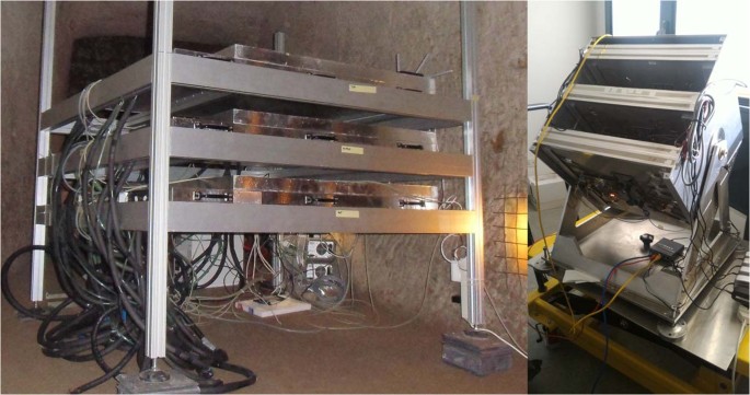
The two muon trackers (called MU-RAY and MIMA) used for the measurements reported in this paper are real-time electronic devices that operate autonomously, with remote control and readout. The basic elements are bars of plastic material doped with a scintillating compound, following a simple and widespread technique for particle detection. The light generated by muons in the plastic scintillator bars is detected by Silicon Photomultipliers (SiPMs). These photosensors, recently developed, are solid-state devices that, as such, do not require any high voltage supply and have a very low power consumption. These features allow us to operate the detectors with relative ease also in remote environments. For a detailed description of the technology we address the reader to ref.https://doi.org/10.1038/s41598-017-01277-3
(2017)." href="https://www.nature.com/articles/s41598-019-39682-5#ref-CR24" data-track="click" data-track-action="reference anchor" data-track-label="link" data-test="citation-ref" aria-label="Reference 24">24 is a planar array of 64 plastic scintillator bars. The section of the scintillator bars has the shape of an isosceles triangle with 3.3 cm basis and 1.7 cm height. A central hole hosts a wavelength shifting optical fibre that carries the light to the SiPM. The scintillator bars were extruded at the NICADD facility of the Fermilab Laboratory. The triangular bars are packed together so that each one is half superimposed to its neighbours. The coordinate perpendicular to the bars is measured with a resolution of about 2 mm. The module is subdivided in two arrays of 32 scintillator bars. Figure 1 shows one of such arrays.
Figure 1
A half module of the MU-RAY muon tracker with its 32 triangular scintillator bars and the 32 wavelength shifting optical fibres that transmit the light to the photosensors.
Two modules with orthogonal bars form a XY plane. The muon trajectories are tracked by a sequence of three XY planes. At Mt. Echia, the distance between the outer planes was 0.50 m. The angular resolution in the measurement of the muon trajectory with this configuration was around 6 mrad. The XY planes have an active area of about 1.0 × 1.0 m. Muons are tracked up to a maximum angle of 60° with respect to the view axis of the tracker, i.e. to the direction perpendicular to the tracker planes. The left side of Fig. 2 shows the MU-RAY tracker at location A.
MIMA29 is a smaller muon tracker basically using the same technique, except that the SiPMs are in direct contact with the scintillator bars (i.e. no wavelength shifter is used). Like the MU-RAY tracker, it consists of three XY planes. The outer XY planes are formed by two orthogonal arrays of 21 scintillator bars. The section of the scintillator bars has the shape of an isosceles triangle with 4 cm basis and 2 cm height. The coordinates of the muons are measured with a resolution of about 3 mm. The outer XY planes are 0.34 m apart. Muon tracking is carried out with an angular resolution of about 14 mrad. The central XY plane, with a coarser structure and formed by scintillator bars of rectangular section, is used as a constraint in muon tracking. However, its use was not required for this measurement. Muons are tracked up to a maximum angle of 45° with respect to the view axis of the tracker. The active area amounts to about 0.4 × 0.4 m (1.0 × 1.0 m for MU-RAY). The right side of Fig. 2 shows the MIMA tracker.
Muon Transmission
Each muon tracker determines the muon trajectories after the traversal of the volume under investigation. The procedure for the analysis of the events with a muon trigger acquired in the data taking runs, in order to select those with a recognizable muon and to reconstruct its track, is described in ref.https://doi.org/10.1038/s41598-017-01277-3
(2017)." href="https://www.nature.com/articles/s41598-019-39682-5#ref-CR24" data-track="click" data-track-action="reference anchor" data-track-label="link" data-test="citation-ref" aria-label="Reference 24">24 for the MU-RAY tracker and in ref.29 for the MIMA tracker.
The muon flux is measured as a function of the elevation angle α and of the azimuth angle ϕ of the track, as defined in the reference system of the tracker itself. The elevation angle (complementary to the zenith angle) is zero in the horizontal direction and 90° at the Zenith.
The muon transmission T(α, ϕ) is defined as the ratio between the muon flux measured underground as described above and the flux measured at the surface in dedicated runs carried out in the laboratory (free sky)https://doi.org/10.1038/s41598-017-01277-3
(2017)." href="https://www.nature.com/articles/s41598-019-39682-5#ref-CR24" data-track="click" data-track-action="reference anchor" data-track-label="link" data-test="citation-ref" aria-label="Reference 24">24. Since no damage to the detectors or change of operating conditions happened during the runs, we assume that the geometrical acceptance, the trigger efficiency, and the selection efficiency are the same in the data samples taken underground and at the surface, effectively cancelling out in the ratio giving the muon transmission. For a detailed mathematical formulation, see the Section Methods or ref.https://doi.org/10.1038/s41598-017-01277-3
The relative transmission R(α, ϕ, ρ) is defined as the ratio between the measured and the expected muon transmission, the latter evaluated by taking into account the absorption of the muon flux in the absence of internal structure such as cavities. The relative transmission equals unity in case no internal structures are present and the correct rock density ρ is inserted in the evaluation of the expected transmission.
The expected transmission was evaluated using the muon flux as a function of energy measured at the surface by the ADAMO experiment30. The muon flux reaching the tracker was evaluated by integrating the flux impinging on the surface above a muon energy threshold that takes into account the energy loss in the rock traversed31. The path length of muons in the rock was obtained using a Digital Terrain Model (DTM) describing Mt. Echia. The DTM was obtained from LIDAR observations elaborated with the software packages Terrasolid - Terrascan, LP360, RIEGL Riscan Pro, Golden Software - Surfer 12 and Roothttps://doi.org/10.1038/s41598-017-01277-3
(2017)." href="https://www.nature.com/articles/s41598-019-39682-5#ref-CR24" data-track="click" data-track-action="reference anchor" data-track-label="link" data-test="citation-ref" aria-label="Reference 24">24. We assumed an uniform density of the rock (tuff at Mt. Echia) and used its best estimate ρ = 1.71 g/cm3, as previously determined from our datahttps://doi.org/10.1038/s41598-017-01277-3
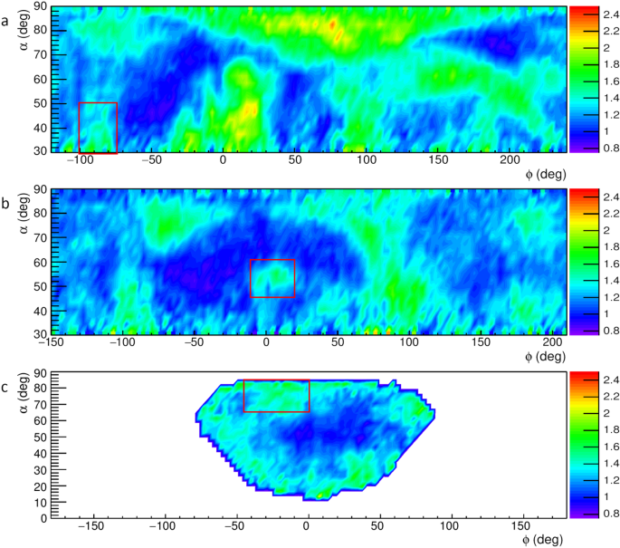
Figure 3 shows the system of known cavities inside Mt. Echia visible from the three muon tracker locations A, B and C (indicated in the figure and at an altitude around 10 m a.s.l.). Figure 4a–c shows the relative transmissions R(α, ϕ, ρ), as measured at the three locations A, B and C of the muon trackers, each one giving a projective muographic image. Regions with high relative transmission (green in the figure) signal the possible presence of cavities.
Figure 3
The system of known cavities and the three locations A, B and C of the muon trackers.
a–c The relative transmission R(α, ϕ, ρ) observed at the locations A, B and C, respectively, in the reference systems of the corresponding muon trackers. The angular regions associated to the hidden cavity are indicated with rectangles. The plot was obtained using the software ROOT and the smoothing tool Contour4 was applied.
(2017)." href="https://www.nature.com/articles/s41598-019-39682-5#ref-CR24" data-track="click" data-track-action="reference anchor" data-track-label="link" data-test="citation-ref" aria-label="Reference 24">24 were obtained with the MU-RAY muon tracker installed at location A. A second set of data was taken immediately afterwards with the same MU-RAY tracker at the location denoted by B. At both locations, the XY planes of the tracker were placed horizontally parallel to the cavern floor, so that the view axis of the tracker was vertically oriented.
(2017)." href="https://www.nature.com/articles/s41598-019-39682-5#ref-CR24" data-track="click" data-track-action="reference anchor" data-track-label="link" data-test="citation-ref" aria-label="Reference 24">24. We focused attention on the (green) signal of high transmission visible near the bottom-left corner, which suggests the presence of a hidden cavity. The high transmissivity region of interest is within an angular boundary indicated by a red rectangle that corresponds to an elevation angle αA in the range of 30° to 50°, and an azimuth angle ϕA in the range of −100° to −75°.
The projection in space of this angular region from location A intercepts the projection from location B of a similar region of high transmissivity that lies within the angular boundary indicated by the rectangle in Fig. 4b. The region corresponds to αB in the range of 45° to 60° and ϕB in the range of −10° to 20°. The muography carried out from location B thus confirmed the presence of a hidden cavity and roughly localized it in space at the intercept of the two projections.
We then took data, using the MIMA tracker, at the location denoted by C in Fig. 3 The view axis of the MIMA tracker was tilted by about 45.5° with respect to the vertical direction and was pointing towards the presumed location of the hidden cavity.
The hidden cavity under investigation is viewed from location C at an angle that is different than that at locations A and B. This choice of the viewing site C effectively allows us to perform a high resolution 3D study in combination with the muographies taken at locations A and B. However, the choice of tracker locations was done compatibly with the logistics of the underground site, where we used pre-existing caves and tunnels. Hence the chosen locations are adequate but not optimal for a 3D muography.
In Fig. 4c a signal for a hidden cavity from location C is seen in the angular region expected from the two previous muographies, This high transmissivity region is contained within the red rectangle, which corresponds to the ranges of 65° to 85° and of −45° to 0° for αC and ϕC, respectively. Actually, the three angular regions indicated by rectangles in Fig. 4a–c all point to the same high transmissivity structure (i.e. a hidden cavity).
The MU-RAY tracker data taking at locations A and B lasted 26 and 8 days, respectively. The numbers of acquired events with a muon trigger were 14 × 106 at location A and 5 × 10⁶ at location B. The MIMA tracker data taking at location C lasted 50 days, corresponding to 5 × 10⁶ muon trigger events. The runs to measure the muon flux on the surface were taken keeping the same orientation of the muon trackers as underground. The run lasted 2 days, corresponding to 12 × 106 acquired muon trigger events for MU-RAY, and 18 days, corresponding to 19 × 106 muon trigger events, for MIMA.
3D reconstruction of the hidden cavity
A clustering algorithm was applied to select regions in Fig. 4a–c with a relative transmission R above a significant threshold value, so that they could be considered as corresponding to cavities. The clustering algorithm was based on the assumption that the distribution of the relative transmission R in Fig. 4a–c has two components. One of the components corresponds to the transmission mostly through solid rock. A second component correspond to cases where voids are encountered by muons. These two components were obtained by fits with Gaussian curves. The component corresponding to transmission through solid rock (essentially determined by the shoulder at low transmission) was used to set the threshold to define the clusters corresponding to the presence of voids. This threshold was set at a value such that the probability to be a solid rock region is smaller than 2.5%. This corresponds to a value of R above 1.51 in the muographies acquired with the MU-RAY tracker (Fig. 4a,b) and to a slightly different value (1.52) for the muography with the MIMA tracker (Fig. 4c).
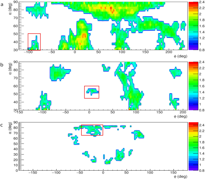
The threshold obtained in this manner is used to search for the “seeds” (i.e. the starting regions) of the clustering algorithm. Subsequent recursive aggregation of points appearing in the 2D muography to each cluster is made by lowering progressively the threshold in R for points which are close in space to existing clusters. Cluster reconstruction stops when no further points (close in space to an existing cluster) have a high-enough value of R (1.37 for MU-RAY and 1.39 for MIMA) to be associated to the cluster. In this second selection the probability for a rock filled bin to exceed the thresholds was higher (16%) but the request of proximity to a signal region ensures a low background. The regions selected by the clustering algorithm are indicated by solid lines in Fig. 5a–c.
Figure 5
Regions in the map of the relative transmission R(α, ϕ, ρ) selected by the clustering algorithm as corresponding to a cavity. The angular regions associated to the hidden cavity are indicated with rectangles. The plot was obtained using the software ROOT and the smoothing tool Contour2 was applied.
In order to reconstruct in space the hidden cavity, we started by defining a grid of points in a cubic volume that encloses the region of space where the cavity is supposed to be, according to the angular ranges defined above. As a general criterion, a point was considered to be located inside a cavity if in each of the three projective muographies it corresponded to a direction lying inside a signal cluster as defined above.
This procedure was tested by simulating the presence of a spherical cavity with 6 m diameter, approximately located at the presumed position of the hidden cavity and having a similar size. The simulated cavity was surrounded by rock using our best estimate of density for Mt. Echiahttps://doi.org/10.1038/s41598-017-01277-3
(2017)." href="https://www.nature.com/articles/s41598-019-39682-5#ref-CR24" data-track="click" data-track-action="reference anchor" data-track-label="link" data-test="citation-ref" aria-label="Reference 24">24 as quoted above in this paper. The minimum cavity size for our experiment sensitivity, was estimated to be 1.5 m over 50 m total rock thicknesshttps://doi.org/10.1038/s41598-017-01277-3
(2017)." href="https://www.nature.com/articles/s41598-019-39682-5#ref-CR24" data-track="click" data-track-action="reference anchor" data-track-label="link" data-test="citation-ref" aria-label="Reference 24">24. The spherical shape was chosen in order to study the effects of the non optimal choice of the trackers’ locations, and in particular to highlight possible ensuing asymmetries.
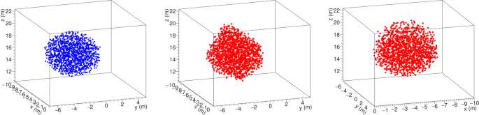
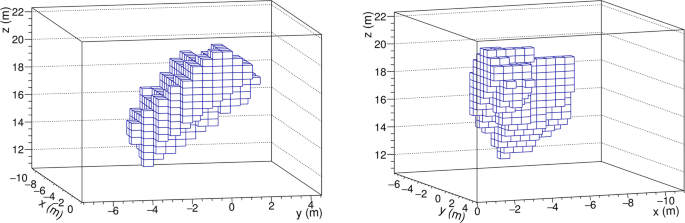
The result of the simulation is shown in Fig. 6. The blue dots in the view on the left side represent an ensemble of points distributed on the grid and located inside the simulated spherical cavity. The points satisfying the triple cluster criterion are denoted by red dots in the two views on the right side of the figure.
Figure 6
The simulated spherical cavity with a 6 m diameter (blue dots, on the left) and two views of its 3D reconstruction (red dots, on the right), in a coordinate system with origin at the centre of the MIMA muon tracker at location C.
The criterion is satisfied also by points that in a projection appear in the shadow of the cavity, rather than inside. The halo that is observed in Fig. 6, extends by about 1 m beyond the cavity. In particular, one can notice a halo upwards, presumably due to fact that the three tracker locations are all at a level considerably lower than the hidden cavity (hence of the spherical cavity). The halo could be reduced by placing the trackers at angles that are more favourable for a triangulation or by increasing the number of trackers locations beyond the minimal number of three used in this work.
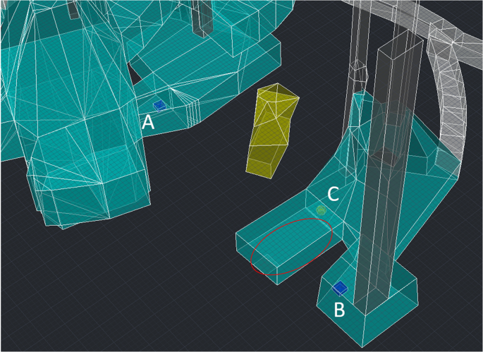
Figure 7 shows two views of the 3D muographic image of the hidden cavity in the reference system associated to the MIMA muon tracker, as obtained following the procedure described above. It appears as an inclined cavity with a width of about 4 m, a height of 3–4 m and a length of about 7 m. Figure 8 shows the hidden cavity inserted in the CAD representation of the known cavities.
Figure 7
Two views of the 3D reconstruction of the hidden cavity, in a coordinate system with origin at the centre of the MIMA muon tracker at location C.
The 3D reconstruction of the hidden cavity (in yellow) inserted in the CAD model. The ellipse indicates the cavity where debris were found, providing a hint for a hidden cavity above it.
Especially when compared with the single muographies given in Fig. 4a–c, taken as examples of current 2D muographic images, the reconstruction in space of the hidden cavity shown in Fig. 7 demonstrates the power of our approach to 3D muography in identifying, localizing and reconstructing in space hidden cavities in complex systems, resolving the the ambiguities that affect 2D muographies.
Hints for the hidden cavity
The existence of a hidden cavity in the region of space localised by our 3D muography, is consistent with previous hints from surveys carried out on site by one of the present authors (G. Minin), together with personnel of the Bourbon Tunnel. The cavity outlined with the ellipse in Fig. 8 was found to be obstructed by a large quantity of material that could not be removed. The presence of this material suggested the existence of an empty space at a higher altitude, originally belonging to a larger sized structure. Various unsuccessful attempts have been made at finding accesses to the cavity from the top or from the sides. Also unsuccessful were the attempts made at probing the hidden cavity from neighbouring cavities with a ground-penetrating radar (GPR), having a reach limited to about 3 m32.
Presumably, the hidden cavity was originally a quarry from where tuff was extracted to construct a building above it. Subsequently it was probably turned into a cistern, and tied up to branches of the aqueduct dating from the Renaissance. Clues have been found, indicating that during the Second World War work had started to access the underground shelters from the surface through a staircase, presumably within this hidden cavity. After the war, the cavity was partially filled with debris, on several occasions.
Outlook
The hidden cavity was reconstructed in space on the basis of its correspondence with the presence of a high muon transmittivity cluster in each of the three projective images. These clusters were defined through the use of algorithms based on setting a threshold in the transmittivity. The technique could be further refined through the development of algorithms that fully exploit the quantitative information carried by the transmittivity.
We also developed and started to apply an innovative technique that allows a first localisation in space already from a single muography33. This technique is based on a stereoscopic principle similar to that of the human sight and is applicable wherever the size of the muon tracker is not negligible with respect to its distance to the structure being investigated. In this case, a rough estimate of this distance can be obtained by projecting backwards the muographic image of the object and minimizing its angular width as a function of the distance of the plane onto which it is projected.
Our group is now planning the study of underground structures in the mountain where the ancient city of Cumae was settled as a Greek colony in the 8th century BC and in the surrounding area of the Phlegraean Fields, very rich of archaelogical remains. The Phlegraean Fields were of primary strategic importance in the Roman times, with the commercial harbour at Puteoli and the military harbour at Misenum. Moreover, Baia was hosting a rich residential and thermal area. In addition, a measurement campaign with MIMA tracker is ongoing inside the Temperino archaeological park, a mine from the Etruscan age located in Campiglia Marittima (Tuscany).
Conclusions
We have developed a new method for a 3D muographic reconstruction directly from the data, exploiting the resolution obtainable with the muographic technique. We have proven the existence of a hitherto unknown cavity inside Mt. Echia, of which only hints were present, and reconstructed its position and shape in space. The search at Mt. Echia was motivated both by the need to investigate an area of potential geological risk and by the curiosity about the history hidden underneath the ancient city of Naples.
Because of its complex system of cavities, Mt. Echia also represents a testing ground fraught with difficulties in which to develop muography techniques for application in the field of archaeology and, in general, in the investigation of hidden structures. Especially in complex situations, our 3D muographic reconstruction method definitely enhances the discovery potential of the technique.
Methods
Muon transmission
For any given angular bin (α, ϕ), the muon transmission T is defined as the ratio between the muon rate observed underground and the rate observed on the Earth surface. The latter is measured in a dedicated run at a surface laboratory without overburdens or overhead structures (free sky run)https://doi.org/10.1038/s41598-017-01277-3
As the muon tracker and its operating conditions are the same at the two locations, most factors (such as the sensitive area of the muon tracker, its angular acceptance, the trigger efficiency and the analysis efficiency) linking the muon rates to the number of recorded events N(α, ϕ) cancel out in the ratio. This is not the case for the data taking time ΔT and for the data acquisition efficiency ϵDAQ(ν), which depends of the trigger rate ν that is much lower underground.
With good approximation the measured muon transmission Tm(α, ϕ) is thus given by
where Φ(α, E) is the differential muon flux impinging on the Earth surface as a function of the muon energy E, which also depends on the elevation angle α and has been measured by the ADAMO experiment30. The lower limit Emin(α, ϕ, ρ) of the integral at the numerator is the minimum energy that muons must have in order to cross the rock overburden and be recorded underground by the muon tracker. It depends on average rock density ρ and on the rock thickness, the latter being given by the DTM for any given (α, ϕ). Emin is evaluated using a model that parametrises the muon energy loss in matter31. The lower limit E0 of the integral at the denominator is the minimum energy required for muons to be recorded by the muon tracker. For the MU-RAY muon tracker it is estimated at about 100 MeV, supposedly independent on (α, ϕ) in the angular range under study. The sensitivity of the expected muon transmission on E0 is such that a value of 200 MeV would result in a transmission higher by at most 4%. The estimate for the MIMA muon tracker is E0 = 170 MeV.
The relative muon transmission R(α, ϕ, ρ) is defined as
and represents for each angular bin, the muon excess (or deficit) for the target under observation when compared to a uniformly homogeneous rock hypothesis.
Clustering algorythm
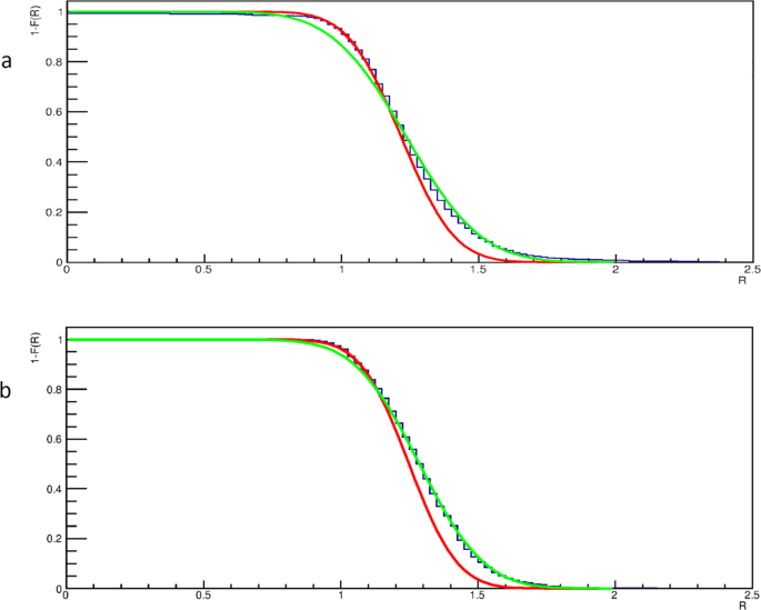
The distribution of the relative transmission R given in each muography of Fig. 4a–c was interpreted as the sum of two components, one corresponding to transmission through rock without voids and another corresponding to transmission through rock with voids. We complement the main text of the paper showing in Fig. 9a,b fits with two Gaussian components. The fits are shown for one of the locations of the MU-RAY muon tracker and for the MIMA muon tracker.
Figure 9
Fits of the cumulative distributions of the relative transmission R of the muography taken with the MU-RAY muon tracker at the location B (a) and with the MIMA muon tracker (b). The distributions are fitted by two Gaussian components, one corresponding to transmission through rock without voids (red) and another corresponding to trasmission through rock with voids (green).
This article is an installment of Future Explored, a weekly guide to world-changing technology. You can get stories like this one straight to your inbox every Thursday morning by subscribing here.
For more than 20 years, the International Space Station (ISS) was humanity’s only off-world home, but today, two continuously occupied space stations are orbiting Earth — and the number could increase dramatically in the near future.
The background
After proving in the 1960s that they could send people to space and the moon, the US and the Soviet Union (USSR) shifted their focus in the 1970s to building spacecraft that could serve as temporary habitats for humans in Earth’s orbit.
Once established, these space stations could be used to observe both space and Earth, conduct microgravity research that would be impossible otherwise, and help prepare astronauts for longer missions throughout the solar system.
Both nations launched and crewed smaller, temporary stations in the 1970s, including the US’s Skylab. Following the success of the first permanent station (the USSR’s Mir) in the ‘80s, the Russian and American space agencies teamed up in the ‘90s to build the International Space Station, along with Japan, Europe, and Canada.
The first crew arrived at the ISS in November 2000 — about five months after the last crew left Mir — and the space station has been continuously occupied ever since then, delivering scientific breakthroughs in astronomy, physics, medicine, and more.
It’s starting to show signs of age, though, and in January 2021, NASA announced plans to deorbit the ISS in 2031.
The International Space Station has been continuously occupied since November 2000.
Beyond the ISS
For two decades, the ISS was the only occupied space station, but in April 2021, China launched the first module of Tiangong, a space station capable of supporting three astronauts. Within two months, it received its first crew and has been occupied ever since.
Today, a handful of new space stations are in development, and unlike in the past, they aren’t all the work of national space agencies. Here are some of the ones most likely to get off the ground in the near future.
Lunar Gateway
Instead of building another space station where the ISS is — about 250 miles up, in low Earth orbit (LEO) — NASA has teamed up with Canada, Europe, and Japan’s space agencies to build one near the moon, nearly 240,000 miles away.
NASA plans to begin assembling this space station, dubbed the Lunar Gateway, in 2024, and it expects it to play a pivotal role in its plans to maintain a human presence on the moon and eventually send astronauts to Mars and beyond.
“Through Gateway, NASA is extending more than 20 years of discovery, research, and international collaboration in low Earth orbit to deep space, starting at the moon,” said Dan Hartman, Gateway Program manager.
An artist’s concept of the Lunar Gateway. Credit: NASA
Russian Orbital Service Station
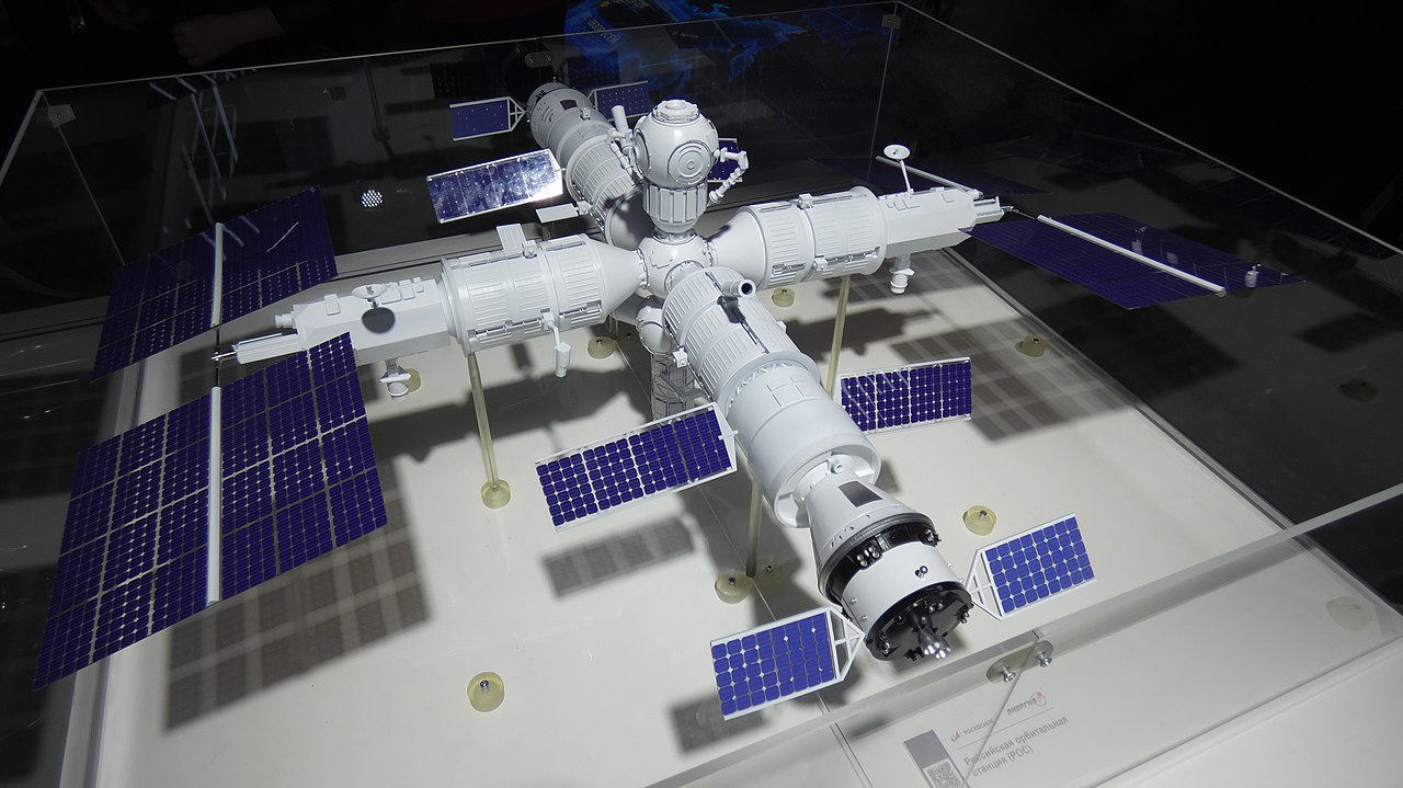
In 2022, Russia announced that it would be pulling out of the ISS in 2024 in order to focus on building its own habitat in LEO, the Russian Orbital Space Station (ROSS).
Russia’s current plan is to build ROSS in two stages, with the first launching sometime between 2025 and 2030 and the second between 2030 and 2035. After the first stage launches, Russia will begin sending crew to the space station for extended stays twice per year, rather than keeping it permanently occupied.
A model of the ROSS space station. Credit: Kirill Borisenko / Wikimedia Commons
ISRO Space Station
India’s space program isn’t quite as capable as the US, Russia, or China’s, but the nation is currently preparing to launch its first crewed mission to space in 2024 and has plans to start building its own space station in 2035.
This station is expected to be small, weighing just 22 tons, compared to the ISS’s more than 440 tons, and India envisions astronauts occupying it for just 15 to 20 days at a time.
Once India completes its first crewed space mission, it plans to turn its attention to building a space station. Credit: ROSCOSMOS
Going commercial
While NASA doesn’t plan to build another space station in LEO, it is helping several private companies develop their own space stations closer to home.
One of those companies, Axiom Space, received a NASA contract in 2020 to build up to four modules that could attach to the ISS as soon as 2025 and then detach to orbit freely once the ISS deorbits.
The following year, NASA announced that it was giving three companies — Nanoracks, Blue Origin, and Northrop Grumman — a total of $415 million to build their own commercial space stations in LEO. Those are all scheduled to be ready for habitation by 2030.
“My attitude is if you pay your rent and you don’t break my space station then I’m happy.”
BRENT SHERWOOD
The idea is that NASA will be able to rent space aboard one or more of these stations after retiring the ISS in 2031. Meanwhile, the owners of the stations will also be able to serve other customers interested in accessing space.
“It’s like a traditional business park,” Brent Sherwood, Blue Origin’s director of advanced development programs, told TIME in 2022. “We do the utilities — the sewers, the power lines, all the stuff that makes it usable.”
“The tenants have their own business model, whatever it might be — maybe a filmmaker or a national laboratory or a space agency,” he continued. “But my attitude is if you pay your rent and you don’t break my space station then I’m happy.”
A rendering of Blue Origin’s Orbital Reef space station. Credit: Blue Origin
Though it doesn’t have the backing of NASA, Airbus — the world’s largest manufacturer of airliners — is also developing a tri-level space station, “LOOP,” that it sees as a viable replacement for the ISS.
This swanky space station concept has room for four to eight astronauts and features a greenhouse, a science deck, and a centrifuge level to simulate gravity conditions.
“The Airbus LOOP is designed to make long-term stays in space comfortable and enjoyable for its inhabitants, while supporting efficient and sustainable operations at the same time,” Airbus said in a statement.
The big picture
It’s not yet certain that any of these other space stations will come to fruition, and it’s even less certain whether the market for space access will be large enough to support all of the commercial ones if they do launch.
“I would love to be optimistic and say, yes, all four are going to be hugely successful, but the market is what’s going to drive this,” Rick Mastracchio, Northrop Grumman’s director of business development, told TIME.
Still, the more space stations we have in orbit around Earth or the moon, the more opportunities there will be for off-world tourism, entertainment, manufacturing, and scientific research — the kind that could one day help us establish space stations throughout the solar system.
We’d love to hear from you! If you have a comment about this article or if you have a tip for a future Freethink story, please email us at tips@freethink.com.
Since there will be more space stations orbiting our planet Earth in the next few decades, Space Archaeology will continue to grow rapidly as each new Space Station will use a more advance version of the remote sensing technology or a different technology all together when searching for archaeological sites. The ISS (International Space Station) has been using remote sensing technology to search for archaeological sites however it will retire some time in 2031 as mentioned in the article.
The current International Space Station orbits earth at a distance of roughly 250 miles up. NASA is planning for the next Space Station to orbit the moon – roughly 240,000 miles from earth. This planned Space Station, called Lunar Gateway, will be a joint effort with Canada, Europe and Japan. You can read all about it here:
When we look at Mesoamerican structures we primarily see the last time it was built. What we see are the last group of people that inhabited the site. There have been actually various groups of people that have 'come' and 'gone' leaving only some remnants behind of who they were. When a society overthrows another group or when an abandoned ruin is discovered, the new arrivals begin to stack new blocks of rocks on top of the older building. This is evident in their well known buildings that were constructed more than once. Each successive group makes the structure bigger and different than the previous ones before. The pyramid of the Sun and Moon at Teotihuacan were built several times, while Uxmal was built 3 times as told by the oral traditions however scientist have shown that it was built 5 times and Cholula, the largest pyramid, was built at least 6 times. There are several more structures that were built multiple times throughout Mesoamerica.
I posted this thread in this topic in May 2020 and you could find it in page 10.
I reposted it back up here because this commonly accepted theory on how and why Mesoamericans built their structures on top of older structures is now being challenge by another theory as shown in the video below.
Please scroll to 14:09 in the video. The narrator said," that sometimes when a calendar cycle is completed, that is 52 years, the Mayans built a new temple on top of the previous one, therefore under the interior pyramid there is even an older temple...."
Chichen Itza ( El Castillo )
Cholula
What do you people in here think about this other theory?
And which theory of building a new structure or temple on top of an older structure or temple is correct or made more sense to you?
With more research we will eventually find out which theory is correct.
Personally I think that both theories are correct and here's why.
1. If the original Mesoamericans never left the location or were never conquered by the newly arrivals, then they themselves would likely have built a new structure on top of the older structure base on the calendar cycle.
2. On the other hand, if the original Mesoamericans actually abandoned their location or were conquered by the newly arrived Mesoamericans, then it is likely that the newly arrivals were the actual people that built the new structure on top of the older structure.
As you browse the 1529 World Map you will recognize a Christian/ Catholic Cross on the eastern side of Canada.The Holy Cross suggest a religious connection that goes back in time to the Renaissance Era in Europe or possibly earlier.
Questions:
Why was the Holy Cross intentionally placed there?
And why was there only a single Holy Cross found on the World Map?
Excellent facsimile of this important world map recording the voyage of Giovanni de Verrazzano in 1524.
The map includes a depiction of the mythical Sea of Verrazzano stretching from the Pacific to the East Coast of North America.
The map is currently in the Vatican Library. It was previously in the Museo Borgia of the Propaganda Fide.
For a more in-depth treatment, see the My Old Maps
Here's another article concerning Giovanni da Verrazzano's travels and maps.
Please continue browsing the 1529 World Map and you will also see Temistitan, an Aztec capital that we know historically as Tenochtitlan which is located in the Mesoamerican Region. The city was drained and leveled in 1521 and today we know it as Mexico City.
Here's another article on Temistitan that shows a close-up map with more details along with a description of the city.